Process engineering & scale-up Textbook equationsEducational simulationsPlanned pilot train
An extract becomes a reproducible ingredient when heat, mass and momentum transfer are controlled, from flask to plant
How a laboratory extraction changes at plant scale: balances, transport physics, process safety and quality by design. Scale-up rules and technology transfer are on the scale-up page.
Status. EUTECNIQ owns no pilot plant and has run no batches; pilot extraction, solvent recovery and drying are planned for Phase II (facility plan, October 2026). Calculators are educational simulations, not designs.
11 °Cwhere ethanol's saturated vapor reaches its lower flammable limit, 3.3% in air
78 → 42 °Cethanol's boiling point at 1 atm and under a 20 kPa vacuum
120.2 °Ccondensing temperature of saturated steam at 200 kPa absolute
7dimensionless numbers that carry a laboratory result to plant scale
Reference equations of state via CoolProp (agree with the NIST WebBook); NIOSH Pocket Guide, ethanol; Bird, Stewart and Lightfoot, Transport Phenomena, 2nd ed. (2002).
What this page answers
Most scale-up failures come from physics that the laboratory hides: slower heating, coarser particles, longer mixing and the cost of recovering solvent
Process engineering predicts these differences, designs around them and proves the result in pilot runs.
Moving one recipe from a 1 L flask to a 4 m³ vessel slows heating and diffusion about sixteenfold, while mixing stays in secondsModel output, default inputs
Computed with the equations and default inputs of the scale-up calculator below: extraction at 60 °C, steam at 120 °C, U = 500 W/(m²·K), vessel height equal to diameter with jacket area 1.25πT², 60% w/w ethanol, Deff = 10⁻¹¹ m²/s, Rushton turbine (Po = 5, D/T = 0.33) at 400 rpm in the flask and constant power per volume at scale. Bergman et al. 2011; Crank 1975; Grenville and Nienow 2003; latent heats 837 and 2,257 kJ/kg (NIST). Illustrative inputs, not plant data.Text version of the four effects
Heating slows. The time constant Mcp/UA grows with the cube root of volume. Jacket area per volume falls from 46 m²/m³ (1 L) to 2.9 m²/m³ (4 m³), and heat-up from 20 to 60 °C takes about 69 s in the flask and 19 min in the vessel.
Diffusion lengthens. The diffusion time R²/Deff rises with the square of particle size: 0.5 mm particles give 1.7 h, the plant's 2 mm particles 28 h, sixteen times longer.
Mixing slows, but stays short. At constant power per volume the impeller slows from 400 to 63 rpm and the blend time θ95 rises from 4.2 s to 26 s, still seconds against hours of diffusion.
Solvent costs heat. A flask can use 20 kg of solvent per kg of herb; the plant uses 8. Recovering it takes 28 MJ and 11 MJ of latent heat per kg of herb, while the one-stage equilibrium limit falls from 96% to 90%.
Explanation, details and sources
EUTECNIQ would
Close mass and energy balances
Measure scale-dependent parameters in pilot runs
Write transfer packages: ranges, controls, records
Lead hazard analyses with qualified engineers
Proposed
Qualified partners would
Provide pilot or commercial capacity first
Do detailed engineering, fire-code and electrical classification
Fabricate and qualify equipment
External partner
EUTECNIQ does not claim
Equipment, batches, yields or process data
That any calculator here is a validated design
Regulatory approval of any process
Limits
Founder background
Process engineering is the founder's own discipline
A doctorate in computer-aided molecular and process design, early papers on solvent extraction in rotating-disk contactors, pilot scale-up and process modeling at Yazaki, and, as reported by the founder, leadership of plant process engineering for a $140M cGMP expansion at MilliporeSigma. These are prior-employer roles, not EUTECNIQ results (founder page).
Founder-reportedPublications verified
An educational simulation≠a validated industrial design
A laboratory yield≠a plant yield
A P&ID-style schematic≠an engineered, code-reviewed design
Laboratory feasibility≠commercial demonstration
From laboratory to plant
The same recipe gives a lower yield and more degradation at plant scale, unless the process is redesigned around heat transfer, particle size and solvent recovery
Governing relationsheat-up: th = McpUA lnTs − T0Ts − T extraction: F(τ*), sphere in a limited bath τ* = ∫D(T)dt / R² mixing: θ95 = 5.2 (T/D)² / (N Po1/3)
Batch temperature and extraction progress, flask versus plantEducational simulation
Laboratory flask versus plant vessel for the same recipe
Quantity
1 L flask
Plant
What drives the difference
Working volume
Scale
Particle diameter
Plants mill coarser so the marc can be filtered
Solvent per kg herb
Every kilogram of solvent has to be evaporated again
Heat-up to extraction temperature
Jacket area per volume falls as V−1/3
Cool-down to 35 °C
Same physics, in reverse
Mixing time θ95 at constant power per volume
Slower impeller at scale; still short against diffusion
Equilibrium limit of one stage
Solvent ratio: less solvent leaves more solute behind
Extracted at the end of the batch
Particle size (diffusion time ∝ R²) and the equilibrium limit
Heat-labile marker degraded
Longer time near temperature during heating and cooling
Solvent to recover per kg extract
Solvent ratio divided by yield
Latent heat to recover it, per kg extract
The largest energy cost of a solvent process
Heat to warm the batch, per kg extract
Thermal mass of solvent and herb
Lower bound of the mass-transfer Biot number, Bi = kfR/Deff ≥ DL/Deff = 100 with no convection at all (Sh = 2). Because Bi ≫ 1, diffusion inside the particles, not agitation, limits extraction at both scales.
Sphere in a well-stirred solution of limited volume: Crank J. The Mathematics of Diffusion. 2nd ed. Oxford: Clarendon Press; 1975, eq. 6.30. Batch heating: Bergman et al. 2011. Blend time: Grenville RK, Nienow AW, in Paul EL, et al., eds. Handbook of Industrial Mixing. Wiley; 2003:507–542. Ethanol latent heat 38.56 kJ/mol at 351.5 K: NIST Chemistry WebBook. All inputs and fixed constants are illustrative.
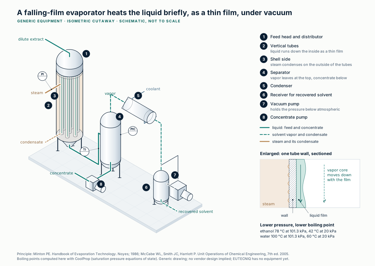
A falling-film evaporator runs the extract down heated tubes as a thin film and works under vacuum, so the solvent is recovered at a lower boiling temperatureSchematic · computed boiling points
Principle: Minton PE. Handbook of Evaporation Technology. Noyes; 1986; McCabe WL, Smith JC, Harriott P. Unit Operations of Chemical Engineering, 7th ed. 2005. Boiling points computed with CoolProp. Generated illustration, EUTECNIQ; generic, no vendor design. Full-size SVGMethod, assumptions and limits
What it calculates
For one recipe at two scales: the batch temperature history, the fraction of extractable solids in solution, the loss of a heat-labile marker, the mixing time, and energy per kilogram of extract for heating and for solvent recovery.
Equations
Vessel: cylinder with liquid height equal to diameter, jacket on wall and flat bottom, A = 1.25πT². Heating with steam at 120 °C from 20 °C, then a hold, then cooling with 20 °C water to 35 °C, each segment exponential with time constant Mcp/UA. Extraction: F = (α/(1+α))·[1 − Σ 6α(1+α) e−qn²τ*/(9 + 9α + qn²α²)], with tan qn = 3qn/(3 + αqn²) and α = solvent-to-particle volume ratio; τ* = ∫D(T)dt/R², exact for a diffusivity that changes in time but not in space. D(T) and the degradation rate k(T) follow Arrhenius laws. Blend time: Grenville and Nienow correlation, impeller speed scaled at constant power per volume.
Variables and units
Solvent 60% w/w ethanol, 900 kg/m³, cp 3.4 kJ/(kg·K); herb cp 1.5 kJ/(kg·K), particle density 1,000 kg/m³, extractable solids 18% of herb; U = 500 W/(m²·K); diffusion activation energy 20 kJ/mol; marker degradation 0.2% per minute at 60 °C with 80 kJ/mol activation energy; liquid diffusivity 10⁻⁹ m²/s; Rushton turbine, Po = 5, D/T = 0.33, 400 rpm in the flask. Latent heats 837 kJ/kg (ethanol) and 2,257 kJ/kg (water), mass-weighted.
Assumptions
One well-mixed stage; partition coefficient 1; uniform spherical particles; no washing of the marc; extract solution not cooled before filtration beyond the stated cool-down; heat of mixing and sensible heat of evaporation ignored.
Valid range
Plant 0.1–10 m³; particles 0.5–5 mm; 4–20 kg solvent per kg herb; 40–80 °C; 15–240 min hold; diffusivity 10⁻¹² to 10⁻¹⁰ m²/s at 60 °C. Very short times use the short-time limit of the series.
What it does not establish
It does not predict a yield for any real botanical. Plants recover yield with countercurrent stages (see the Kremser calculator) and recover energy with multiple-effect or vapor-recompression evaporation; neither is modeled here. Real particles are not spheres, and real constituents degrade by several routes.
Verification
An independent Python reference in tests/numerics/ref/technologies-process-engineering.py solves the diffusion equation in the sphere and bath numerically in real time (method of lines, scipy), without the series or the transformed time, and is checked against the page.
Explanation, details and sources
One recipe runs in a 1 L flask (fine grind, generous solvent) and in a plant vessel with the coarser grind and leaner solvent ratio that filtration and energy cost force. Change the plant settings to see which effect dominates.
Flow diagram and balances
One planned pilot train, its mass and energy balances, and the utilities it would draw on
Nineteen numbered streams: solvent outweighs herb eight to one, and the dried extract is 1% of the mass that movesIllustrative example
Process flow diagram drawn after ISO 10628 conventions; equipment classes and tags as in the pilot-train schematic below; no sizes are specified and nothing has been purchased. Assumptions: 60% w/w ethanol at 8 : 1 solvent to herb; 18% of herb mass extractable; the marc retains 1,200 kg of solvent, of which ethanol is fully and water partly recovered; 30 kg ethanol lost at vents; the resin binds 96 of 180 kg extracted solids; powder leaves at 4.0% moisture. Every unit balances in total mass, solids, ethanol and water; the figure's generator checks this at build time.
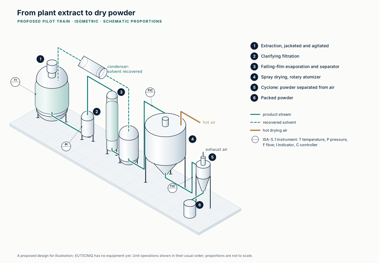
In the proposed pilot train, extract moves from extraction through filtration, evaporation and spray drying to packed powder, and the evaporator returns solvent for reuseProposed design · schematic
Generated isometric drawing, EUTECNIQ. Unit operations in their usual order; instrument tags per ISA-5.1. Proposed design for illustration; no equipment has been selected and proportions are not to scale. Full-size SVGStream table as text (kg per 1,000 kg dry-herb batch)
9 · Solvent vapor, marc desolventizing → solvent recovery
1,080
0
720
360
10 · Spent marc
940
820
0
120
11 · Wash water → C-101
400
0
0
400
12 · Eluent, 70% ethanol → C-101
500
0
350
150
13 · Wastewater, C-101 →
1,084
84
0
1,000
14 · Eluate, C-101 → concentrator E-103
596
96
350
150
15 · Recovered eluent, E-103 →
356
0
350
6
16 · Dryer feed, E-103 → spray dryer D-101
240
96
0
144
17 · Extract powder, D-101 →
100
96
0
4
18 · Water vapor to exhaust, D-101 →
140
0
0
140
19 · Vent loss, solvent recovery →
30
0
30
0
Powder yield 10.0% on dry herb (100 kg per 1,000 kg); 99.4% of the 4,800 kg ethanol charge recovered, 30 kg lost at vents; 90.6% of the 8,000 kg solvent charge returned from recovery; 1.0% of the 9,900 kg that moves through the train leaves as product.
Recovering solvent takes about 31 times the latent heat the spray dryer needs, and water carries most of itIllustrative example
Masses from the illustrative stream table. Ethanol 38.56 kJ/mol at 351.5 K (Majer and Svoboda, via NIST Chemistry WebBook) = 837 kJ/kg; water 2,257 kJ/kg at 100 °C. Heat of mixing and sensible heat are ignored. Multiple-effect evaporation or vapor recompression would cut the steam needed for this duty.Text version: latent heat by recovery step
Latent heat to recover solvent per illustrative batch
Recovery step (per 1,000 kg herb batch)
Ethanol (kg)
Water (kg)
Latent heat (MJ)
Evaporator E-101 (extract)
4,080
2,120
8,200
Marc desolventizing
720
360
1,415
Eluate concentrator E-103
350
6
306
Total solvent recovery
5,150
2,486
9,921
For comparison: water removed in the spray dryer
0
140
316
About 99 MJ of latent heat per kilogram of powder goes into solvent recovery in this example, roughly thirty times the latent heat the spray dryer needs. Table regenerated by src/modules/process/compute/static_tables.py.
Eight unit operations, with a control loop on each variable that sets product quality
Hover or tab to a unit for its operating principle; the descriptions are also listed below.
Planned pilot train: milling, extraction, filtration, evaporation with solvent recovery, resin purification and spray dryingIllustrative schematic
Drawn to ANSI/ISA-5.1 conventions: a circle is a field instrument, a circle in a square a control-system function, a dashed line a signal. Tags follow the ISA letter code (first letter = measured variable: T temperature, P pressure, L level, F flow, A analysis; following letters = function: I indicate, C control, T transmit, D differential). Equipment classes, tags and loop numbers are illustrative; no sizes are specified and nothing has been purchased. Source: ANSI/ISA-5.1-2024, Instrumentation and Control Symbols and Identification.Show unit descriptions
M-101 Hammer mill. Size reduction. Particle size sets the diffusion path, and the time to a given extraction yield scales with the radius squared (see Science lab). Design variables: screen size, rotor speed, feed rate. Too fine a grind slows filtration and heats the material.
R-101 Jacketed, agitated extractor. Solvent dissolves the soluble constituents; temperature, time, solvent ratio and agitation set yield and composition. Nitrogen blanket for the flammable solvent. Design variables: working volume, jacket area, impeller type and speed, temperature range.
F-101 Filter. Separates spent plant material (marc) from the extract. Pressure drop rises as the cake builds (PDI-102). Filter area and media are sized from pilot filtration tests.
E-101 Falling-film evaporator. Liquid runs down heated tubes as a thin film: short residence time and, under vacuum, a low boiling temperature, which suits heat-sensitive extracts. Steam condenses on the shell side. Design variables: area, wetting rate, pressure, steam temperature.
V-101 Vapor–liquid separator. Disengages solvent vapor from the concentrate leaving the evaporator.
E-102 Condenser. Chilled water condenses the solvent vapor so ethanol can be recovered and reused. Duty is set by the vapor rate and its latent heat.
V-102 Solvent receiver. Holds recovered solvent under nitrogen; its ethanol content is checked before it returns to extraction.
VP-101 Vacuum pump. Holds the evaporator and condenser under vacuum (PIC-103); lower pressure lowers the boiling temperature.
C-101 Adsorption-resin column. A macroporous resin binds target constituents from the aqueous concentrate; sugars and salts pass to waste; ethanol elutes the enriched fraction, cut by UV absorbance (AT-105). Design variables: resin, bed volume, loading, flow in bed volumes per hour, eluent strength.
E-103 Eluate concentrator. Removes eluent ethanol and water to reach the dryer's target feed solids.
H-101 Air heater. A steam coil heats filtered ambient air to the dryer inlet temperature (TIC-106).
D-101 Spray dryer. An atomizer makes droplets that dry in the hot air; while water evaporates, evaporative cooling holds each droplet near the wet-bulb temperature. Outlet temperature tracks residual moisture (TIC-107 trims the feed rate). Design variables: inlet and outlet temperature, feed solids, atomization, residence time.
CY-101 Cyclone. Separates powder from the exhaust air by centrifugal force; product leaves through a rotary valve.
BF-101 Bag filter. Captures fines the cyclone misses before the air is exhausted (PDI-108).
K-101 Exhaust fan. Draws air through the dryer train, holding the chamber slightly below atmospheric pressure.
At loop level, the dryer's quality-setting variables each close through a transmitter, a control-system function and a final elementIllustrative schematic
P&ID fragment of the drying section to ANSI/ISA-5.1-2024 conventions. TV-106 is the steam control valve of loop 106; T marks the steam trap. Stream numbers match the process flow diagram above. Not to scale; no vendor design implied.Text version: the eight control loops of the pilot train
Loop
Measures
Acts on
Why it matters for the product
TIC-101
Extractor temperature
Steam valve on the jacket
Extraction rate rises with temperature; so does degradation of heat-labile constituents
PDI-102
Pressure drop across the filter
Operator alarm
A rising drop signals cake build-up or blinding before the filter fails
PIC-103
Evaporator pressure (vacuum)
Vacuum pump speed
Lower pressure lowers the boiling point and the thermal load on the extract
LIC-104
Solvent receiver level
Recycle pump
Holds the recovered-solvent inventory that is returned to extraction
AT-105
UV absorbance at the column outlet
Three-way valve: waste or eluate
Cuts the enriched fraction reproducibly instead of by elapsed time
TIC-106
Dryer inlet-air temperature
Steam valve on the air heater
Sets the drying driving force
TIC-107
Dryer outlet-air temperature
Feed-pump speed
Outlet temperature tracks residual moisture, so feed rate is trimmed to hold it
PDI-108
Pressure drop across the bag filter
Pulse cleaning and alarm
Keeps fines capture and exhaust flow stable
Drawn as flows, the solvent loop dominates: recycled solvent is 7,250 of the 9,000 kg in the extractor
Mass balance per batch (kg), basis 1,000 kg herb, dry basisIllustrative example
Recycled solvent is drawn as its own source on the left and as a return on the right, joined by the dashed loop; a Sankey diagram cannot draw a cycle directly. Assumptions: 60% w/w ethanol at 8:1 solvent to herb; 18% of herb mass extractable; the marc retains 1,200 kg of solvent, of which ethanol is fully and water partly recovered; 30 kg ethanol lost at vents; the resin binds 96 of 180 kg extracted solids; powder leaves at 4.0% moisture. Every node balances in total mass, solids, ethanol and water (a check runs when the page loads).
Spray drying spends roughly half its heat on evaporation; most of the rest leaves in the exhaust air
How it works
The air rate follows from an energy balance on the chamber. A hotter inlet or cooler outlet cuts the air needed per kilogram of water; the outlet temperature also governs residual moisture and heat exposure. The default feed is stream 16 processed over two hours.
Chamber energy balance (reference: ambient air and liquid water at T₀; ΔT = T − T₀)G cH[(1 − f)ΔTin − ΔTout] = E(λ0 + cvΔTout) + P cpΔTout
Water evaporated
Powder made
Dry air required
Inlet air volume
Heater duty
Heat per kg water
Overall thermal efficiency (Masters)
Exhaust dew point (margin)
Where the heater duty goes (kW)Model output
Heat per kilogram of water versus inlet temperatureModel output
ASHRAE Handbook—Fundamentals (2017), ch. 1 Psychrometrics; Masters K. Spray Drying Handbook, 4th ed. (1985), overall thermal efficiency η = (Tin − Tout)/(Tin − T0); NIST Chemistry WebBook (water, 20 °C, 101.325 kPa); Murphy DM, Koop T. Q J R Meteorol Soc. 2005;131:1539–1565.
Method, assumptions and limits
What it calculates
Water evaporated, powder made, dry-air rate, inlet air volume, heater duty and its split, heat per kilogram of water, thermal efficiency and the exhaust dew point.
Equations
Solids balance P = Fxs/(1 − xp); water E = F(1 − xs) − Pxp; the chamber balance above solved for G; heater duty Q = GcHΔTin; humid heat cH = 1.006 + 1.86W0; λ0 = 2,501 − (4.184 − 1.86)T0; exhaust humidity W1 = W0 + E/G; dew point where the Murphy–Koop liquid vapor pressure equals pW1/(0.621945 + W1).
Variables and units
Flows in kg/h; heats in kJ/kg and kJ/(kg·K); duty in kW (kJ/h ÷ 3,600); air volume from the moist-air specific volume 287.05(T + 273.15)(1 + 1.6078W)/101,325 m³ per kg dry air. Each term of the balance is kg/h × kJ/kg = kJ/h.
Assumptions
Steady state; feed enters at ambient temperature; powder leaves at the outlet-air temperature with dry-solids cp 1.5 kJ/(kg·K) (illustrative); wall loss a fixed fraction of heater duty; atmospheric pressure.
Valid range
A solution exists only when (1 − f)ΔTin exceeds ΔTout; otherwise the readouts say "no solution" and a warning explains why.
What it does not establish
Stickiness, glass transition, volatile losses, particle size and residence time, which set the real operating window, are outside the balance.
Verification
Independent Python reference using CoolProp humid-air properties for the dew point, in tests/numerics/ref/technologies-process-engineering.py.
Solvent recovery is the largest energy demand of an ethanol extraction train, so utilities are sized from the mass balance
Each utility is sized from a balance and carries its own safety and quality requirements.
Pressure sets the boiling and condensing temperatures of the solvent recovery loopReference equations of state
Vapor pressures from CoolProp (IAPWS-95 for water; reference equation for ethanol), computed October 24, 2026; 200 kPa steam at 120.2 °C agrees with NIST.Show the table (7 rows)
Blanketing of solvent vessels; inerting a closed-cycle dryer
Vessel volumes and purge rates
Oxygen monitoring; asphyxiation risk in enclosed spaces
Compressed air
Instruments, bag-filter pulse cleaning
Consumers and duty cycles
Oil-free and dry where it touches product
Process water
Extraction, washing, cleaning
Recipe and cleaning volumes
Quality set by specification for each use
Dust collection and ventilation
Milling, powder handling, the dryer exhaust
Capture velocities and air changes
Dust hazard analysis (see process safety below)
Five process solvents against water at 25 °C: ethanol needs 38% of water's latent heat but conducts heat at a quarter of its rateReference equations of state
CoolProp reference equations (IAPWS-95 water; ethanol, methanol, n-hexane, n-heptane), 25 °C and 101.325 kPa; cells are ratios to water. ρ density, μ viscosity, cp heat capacity, k thermal conductivity, ΔHv latent heat at the normal boiling point, pv vapor pressure at 25 °C. Acetone is omitted because CoolProp has no viscosity model for it. Click a column to sort.Data table (absolute values)
Solvent
Density, kg/m³
Viscosity, mPa·s
cp, kJ/(kg·K)
k, W/(m·K)
Latent heat, MJ/kg
Vapor pressure 25 °C, kPa
Boiling point, °C
Water
997.0
0.890
4.181
0.607
2.257
3.17
99.97
Ethanol
785.1
1.082
2.435
0.164
0.850
7.89
78.42
Methanol
786.3
0.544
2.535
0.200
1.101
16.98
64.48
n-Hexane
654.9
0.298
2.273
0.120
0.335
20.16
68.72
n-Heptane
679.6
0.390
2.241
0.122
0.317
6.09
98.38
Latent heats in this table come from the reference equations of state in CoolProp; for ethanol that gives 0.850 MJ/kg, while the solvent-recovery figures above use the measured 38.56 kJ/mol (NIST WebBook), 0.837 MJ/kg. The 1.5% difference changes no conclusion.
Explanation, details and sources
A balance that closes is the first deliverable of a pilot campaign; without it, yield, solvent-loss and residual-solvent claims cannot be trusted. The example is invented but closes on every component.
Transport phenomena
Seven dimensionless numbers decide whether a laboratory observation carries over to the plant
Each number is a ratio of two competing effects; when one changes between scales, the controlling mechanism can changeTextbook definitions
Bird RB, Stewart WE, Lightfoot EN. Transport Phenomena. 2nd ed. Wiley; 2002; Bergman TL, et al. Fundamentals of Heat and Mass Transfer. 7th ed. Wiley; 2011.
Counterflow recovers more heat than parallel flow from the same exchanger, and the gap widens as the exchanger grows
How it works
The effectiveness–NTU method gives outlet temperatures from the conductance UA and the two heat-capacity rates. Here water cools a hot process stream.
Temperature along the exchanger (fraction of heat-transfer area)Model output
Effectiveness versus NTU at the current heat-capacity ratioModel output
Bergman TL, Lavine AS, Incropera FP, DeWitt DP. Fundamentals of Heat and Mass Transfer, 7th ed. Wiley; 2011 (ch. 11, effectiveness–NTU relations). Profiles are integrated from the local energy balances dTh/dx = −(UA/Ch)(Th − Tc) and dTc/dx = ∓(UA/Cc)(Th − Tc).
Method, assumptions and limits
What it calculates
Heat duty, outlet temperatures, effectiveness and the log-mean temperature difference of a two-stream exchanger in counterflow or parallel flow, and the same duty for the other arrangement.
Equations
Counterflow ε = (1 − e−NTU(1−Cr))/(1 − Cre−NTU(1−Cr)), and NTU/(1 + NTU) when Cr = 1; parallel ε = (1 − e−NTU(1+Cr))/(1 + Cr); Q = εCmin(Th,in − Tc,in); the profiles integrate the local balances with a fourth-order Runge–Kutta step.
Variables and units
Flows in kg/h (÷ 3,600 to kg/s); heat capacities in kJ/(kg·K); C = ṁcp in kW/K; UA in kW/K on a logarithmic slider from 0.2 to 20; temperatures in °C; duty in kW.
Assumptions
Constant U and heat capacities; no phase change; no heat loss; water cp 4.18 kJ/(kg·K); the process-stream heat capacity is an illustrative input (ethanol–water mixtures lie below water). Fouling would lower U over a campaign; design adds a fouling resistance.
Valid range
Single-phase liquids within the slider ranges. The UA·ΔTlm check equals the duty to rounding.
What it does not establish
Exchanger area, pressure drop, fouling margin or mechanical design.
Verification
An independent Python reference integrates the two differential energy balances numerically (scipy) and compares outlet temperatures with the page, in tests/numerics/ref/technologies-process-engineering.py.
A 2,000 L batch takes about thirteen times as long to heat as 1 L, because jacket area per liter falls as volume rises
How it works
With condensing steam in the jacket, a well-mixed batch approaches the steam temperature exponentially, with a time constant M cp/UA that grows with the cube root of volume for similar vessels.
Batch heating with an isothermal heating mediumT(t) = Ts − (Ts − T0) × exp(−UA tM cp)
1 L to target
100 L to target
2,000 L to target
Jacket area per liter, 1 L → 2,000 L
Batch temperature versus time at three scalesModel output
Time to target versus batch volume (log–log): slope one-thirdModel output
Bergman et al. 2011, lumped-capacitance energy balance; Perry's Chemical Engineers' Handbook, 9th ed. (2018), batch heating of agitated vessels; NIST Chemistry WebBook, saturation properties of water.
Method, assumptions and limits
What it calculates
The time for a well-mixed batch to heat from its starting temperature to a target with condensing steam in the jacket, at 1 L, 100 L and 2,000 L.
Equations
T(t) = Ts − (Ts − T0)e−t/τ, τ = Mcp/(UA); time to target t = τ ln[(Ts − T0)/(Ts − T)]; vessel diameter T = (4V/π)1/3, jacket area 1.25πT².
Variables and units
U in W/(m²·K); M = 998V kg; cp = 4,184 J/(kg·K); A in m²; τ in s.
Assumptions
Cylindrical vessels with liquid height equal to diameter, jacket on the wetted wall and a flat bottom, geometrically similar across scales; constant U (an illustrative input); water-like contents (998 kg/m³, 4.18 kJ/(kg·K)), well mixed; no heat loss. Saturated steam at 200 kPa absolute condenses at 120.2 °C (NIST).
Valid range
Target temperature below the steam temperature (the target is held at least 0.5 K below it).
What it does not establish
Real U depends on agitation, fouling and the jacket side; internal coils change the area-to-volume ratio.
Verification
Independent Python reference in tests/numerics/ref/technologies-process-engineering.py.
Time to target across batch volume and overall coefficient UModel output
Volume and time are on logarithmic axes. Amber marks heat-up within 60 minutes. Points mark 1 L, 100 L and 2,000 L at the U set above; the steam, starting and target temperatures follow the sliders.
Show data (minutes to target)
Volume
U = 100
250
500
1,000
1,500 W/m²·K
The table fills in when the page's scripts run; the equation above gives every value.
Same equation and assumptions as the calculator above: geometric similarity, liquid height equal to diameter, jacket on the wetted wall and bottom, water-like contents, constant U. Heat-up time scales as V1/3/U, so a tenfold larger U offsets a thousandfold larger volume.
Three ideal countercurrent stages at a solvent ratio of 1.5 recover 88% of the solute, and each added stage buys less
How it works
Fresh solvent meets the most exhausted material, so every stage keeps a concentration difference. The Kremser equation gives the fraction left after N ideal stages; the solvent ratio S also sets the evaporation load downstream.
Kremser equation, countercurrent washing (stripping form)φ = S − 1SN+1 − 1 recovery = 1 − φ S = VL
Solute recovered
Left in the marc
Stages for 99% at this S
Adding one more stage
Solute recovered versus number of ideal stagesModel output
Ideal stages needed versus solvent ratio: solvent and stages trade against each otherModel output
Kremser A. Theoretical analysis of absorption process. National Petroleum News. 1930; Seader JD, Henley EJ, Roper DK. Separation Process Principles, 3rd ed. Wiley; 2011 (Kremser method; leaching and washing).
Method, assumptions and limits
What it calculates
The fraction of solute recovered after N ideal countercurrent washing stages at solvent ratio S, the stages needed for 99% and the gain from one more stage.
Equations
Fraction left in the marc φ = (S − 1)/(SN+1 − 1), and 1/(N + 1) when S = 1; recovery = 1 − φ.
Variables and units
S = fresh solvent flow ÷ retained solution flow (dimensionless); N whole number.
Assumptions
Ideal stages (overflow and retained solution leave at the same concentration); constant underflow (retained solution per kg of solids); solute already dissolved; solute-free fresh solvent.
Valid range
S 0.5–4, N 1–10; with S < 1 recovery approaches S and 99% may be unreachable, which the readout states.
What it does not establish
Diffusion out of particles makes real stages less than ideal; stage efficiency is measured in pilot runs.
Verification
An independent Python reference solves the stage-by-stage solute balances as a linear system (numpy) instead of using the closed form, in tests/numerics/ref/technologies-process-engineering.py.
In drying, heat supply to the surface limits the constant-rate period and moisture moving out of the solid limits the falling-rate period
How it works
Above the critical moisture content the surface stays wet and dries at a rate set by the air. Below it, internal transport limits the rate, so the last few percent of moisture take most of the time.
Drying time, constant rate then linear falling ratetc = Ls(X0 − Xc)A Nc tf = Ls(Xc − Xe)A Nc lnXc − XeX − Xe
Constant-rate period
Falling-rate period
Total to target
Drying-rate curve and moisture versus timeModel output
Total drying time versus target moisture: the last few percent cost the mostModel output
Geankoplis CJ. Transport Processes and Separation Process Principles, 4th ed. Prentice Hall; 2003 (drying of process materials); Perry's Chemical Engineers' Handbook, 9th ed. (2018), solids drying.
Method, assumptions and limits
What it calculates
Constant-rate and falling-rate drying times for a tray or bed to reach a target moisture.
X in kg water per kg dry solid; Nc in kg/(m²·h); Ls/A in kg dry solid per m²; times in h. (kg/m²)(kg/kg)/(kg/(m²·h)) = h.
Assumptions
Constant air conditions; falling rate linear in X − Xe; drying from the exposed surface. Drying droplets show analogous stages, on time scales set by droplet size and air conditions (see the drying page).
Valid range
The critical moisture is held at least 0.05 below the initial moisture and the target at least 0.005 above equilibrium; a warning appears when a slider is clamped.
What it does not establish
Real materials can show several falling-rate zones, shrinkage and case hardening; drying curves are measured.
Verification
Independent Python reference integrating dX/dt with scipy, in tests/numerics/ref/technologies-process-engineering.py.
A concentrated extract can flow laminar where water would be turbulent, which changes pressure drop, pump choice and cleanability
How it works
The Reynolds number decides the flow regime; only in turbulent flow does wall roughness change the friction factor. Raise the viscosity toward a concentrate and the operating point crosses the Moody chart's transition zone.
Darcy–Weisbach with the Colebrook and Haaland friction factorsΔp = fLDρ v22 Re = ρ v Dμ 1√f = −2 log10(ε/D3.7 + 2.51Re √f) laminar (Re < 2,300): f = 64/Re
Velocity
Reynolds number · regime
Friction factor (Colebrook · Haaland)
Pressure drop
Head loss
Pump shaft power
Moody chart computed from the Colebrook equation, with the current operating pointModel output
System curve: pressure drop versus flow rate for the current pipe and fluidModel output
Moody LF. Friction factors for pipe flow. Trans ASME. 1944;66(8):671–684; Colebrook CF. J Inst Civ Eng. 1939;11(4):133–156; Haaland SE. J Fluids Eng. 1983;105(1):89–90; NIST Chemistry WebBook (water at 20 °C).
The Colebrook friction factor over Reynolds number and roughness: in the amber region only roughness mattersModel output
Colebrook CF. J Inst Civ Eng. 1939;11(4):133–156, solved by iteration; Moody LF. Trans ASME. 1944;66(8):671–684. The marked point follows the pipe-flow calculator. Drag to rotate.Data table: Darcy friction factor
Re
ε/D 10⁻⁶
10⁻⁴
10⁻³
10⁻²
0.05
Method, assumptions and limits
What it calculates
Velocity, Reynolds number, friction factor, pressure drop, head loss and pump shaft power for flow in a straight pipe.
Equations
Re = ρvD/μ; laminar f = 64/Re below Re 2,300; otherwise Colebrook 1/√f = −2 log10(ε/(3.7D) + 2.51/(Re√f)), solved by iteration from the Haaland estimate; Δp = f(L/D)(ρv²/2); head = Δp/(ρg); shaft power = QΔp/η.
Variables and units
Flow 1–1,000 L/min (logarithmic slider); D in mm; L in m; μ 1.002–500 mPa·s (logarithmic); ρ in kg/m³; roughness 0.0015–0.5 mm (logarithmic); Δp in Pa: (m/m)(kg/m³)(m/s)² = Pa.
Assumptions
Newtonian fluid; fully developed flow in a straight circular pipe; fittings counted as equivalent length; default fluid water at 20 °C (998.2 kg/m³, 1.002 mPa·s, NIST). The roughness range starts at drawn tubing, 0.0015 mm (Moody 1944).
Valid range
Transitional flow (Re 2,300–4,000) is flagged because the friction factor there is uncertain.
What it does not establish
Concentrated extracts are often shear-thinning and need measured rheology; pump selection also needs NPSH and the pump curve.
Verification
Independent Python reference solving Colebrook with scipy root finding, in tests/numerics/ref/technologies-process-engineering.py.
A continuous step with a broad residence-time distribution under-processes some material and over-exposes the rest
How it works
In continuous equipment, material does not all spend the mean residence time τ inside. In a chain of N well-mixed tanks, one tank gives the broadest spread and many approach plug flow; the equivalent Péclet number describes the same spread for a pipe.
Exit-age distribution E(θ) for tanks in seriesModel output
Danckwerts PV. Continuous flow systems: distribution of residence times. Chem Eng Sci. 1953;2(1):1–13; Levenspiel O. Chemical Reaction Engineering. 3rd ed. Wiley; 1999 (tanks-in-series and closed-vessel dispersion models). Shaded: leaves before the minimum time (amber) and stays beyond the maximum (red).
Method, assumptions and limits
What it calculates
The exit-age distribution of N equal well-mixed tanks, the fractions leaving before and after chosen times, and the Péclet number of a closed vessel with the same variance.
Equations
As above, with θ = t/τ; fractions from the cumulative distribution F(θ) = 1 − e−Nθ Σk=0N−1(Nθ)k/k!; Pe solved by bisection.
Variables and units
N whole number; τ in minutes; the time limits as percentages of τ. E is dimensionless.
Assumptions
Steady flow, equal tanks, no bypassing or dead zones; closed-vessel boundary conditions for the dispersion model.
Valid range
1 to 50 tanks; the Péclet equivalence is exact in variance only.
What it does not establish
Real equipment has dead zones and bypassing that this model cannot show; the distribution is measured with a tracer test.
Verification
Independent Python reference using scipy's gamma distribution and root finding, in tests/numerics/ref/technologies-process-engineering.py.
Explanation, details and sources
Number
Definition
Ratio of
Where it matters here
Reynolds, Re
ρvL/μ
inertia to viscous forces
Laminar or turbulent pipe flow; stirred-tank regime (Re = ρND²/μ)
Prandtl, Pr
cpμ/k
momentum to thermal diffusivity
Heat-transfer correlations for jackets and exchangers
Schmidt, Sc
μ/(ρD)
momentum to mass diffusivity
Mass-transfer correlations; about 10³ for small molecules in water
Nusselt, Nu
hL/k
convective to conductive heat transfer
Film coefficients inside the overall coefficient U
Sherwood, Sh
kfL/D
convective to diffusive mass transfer
Film around a particle; Sh = 2 for a sphere in still liquid
Péclet, Pe
vL/D (= Re·Sc for mass)
advection to diffusion
Axial dispersion in continuous equipment; solute crowding in a drying droplet
Biot (mass), Bi
kfR/Deff
external to internal mass-transfer conductance
Bi ≫ 1: diffusion inside the particle controls extraction, so stirring harder does not help
Mixing, homogenization and unit operations
A homogenizer concentrates energy that a stirred tank spreads over hours, and each unit operation separates or disperses by its own mechanism
Stirred-tank scale-up rules and a 3D power-per-volume map moved to the scale-up page.
A valve homogenizer concentrates energy that a stirred tank spreads over hours, and the product heats with every pass
How it works
The pressure drop across a homogenizing valve is an energy density: 1 MPa delivers 1 MJ/m³. A stirred tank's turbulence breaks droplets only down to a size set by the dissipation rate (Hinze 1955), far above nanoemulsion sizes. The smallest eddy (Kolmogorov length) is a first check of shear sensitivity; damage itself is measured.
Energy density · heating · breakupEv = Δp ΔT = Δpρcp ηK = (ν³/ε)1/4 dmax = 0.725 (σ/ρ)3/5ε−2/5
Energy density delivered
Temperature rise per pass
Temperature rise, all passes
Stirred tank: Kolmogorov length
Stirred tank: largest stable droplet
Stirring time for the same energy
Largest stable droplet and smallest eddy versus energy dissipation rateModel output
Hinze JO. AIChE J. 1955;1(3):289–295 (dmax relation and constant 0.725); Kolmogorov microscale as in Paul EL, et al., eds. Handbook of Industrial Mixing. Wiley; 2003. The computed 2.5 K per 10 MPa (water-like product, 1,000 kg/m³ and 4.0 kJ/(kg·K)) agrees with the 2–2.5 °C per 10 MPa reported by Patrignani F, et al. Front Microbiol. 2019;10:246 and Romano E, et al. Int J Mol Sci. 2021;22(18):9896.
Method, assumptions and limits
What it calculates
Energy density and adiabatic temperature rise of valve homogenization; for a stirred tank, the mean dissipation rate, the Kolmogorov length and the Hinze largest stable droplet; the stirring time that would deliver the same energy density.
Equations
As above, with ε = (P/V)/ρ and ν = μ/ρ; stirring time = nΔp/(P/V).
Variables and units
Δp in Pa (Pa = J/m³); ρ = 1,000 kg/m³ and cp = 4.0 kJ/(kg·K) (water-like product); P/V in W/m³ on a logarithmic slider from 10 W/m³ to 10 kW/m³; σ in N/m; μ in Pa·s, logarithmic from 1 to 100 mPa·s. ε in W/kg = m²/s³; lengths in m.
Assumptions
All homogenizer energy ends up as heat in the product (adiabatic); the tank's mean dissipation rate stands in for the local rate, which near the impeller can be far higher; dilute dispersed phase; Hinze's relation holds in the inertial range, when dmax is well above the Kolmogorov length (the readout turns amber otherwise).
Valid range
10–200 MPa; 1–10 passes; 10 W/m³ to 10 kW/m³.
What it does not establish
It does not predict homogenizer droplet size, which depends on valve design, emulsifier adsorption speed and recoalescence, and is measured. Shear-sensitive ingredients need their own damage tests.
Verification
Independent Python reference in tests/numerics/ref/technologies-process-engineering.py.
Four unit operations that make or purify material, drawn from their operating principles
Hover or tab to a component for a short description. Measuring instruments are on the analytical page.
Supercritical CO₂ extraction: above 31.0 °C and 73.8 bar, CO₂ dissolves lipophilic constituents and releases them when the pressure dropsIllustrative schematic
NIST Chemistry WebBook, carbon dioxide phase-change data (critical and triple points); Reverchon E, De Marco I. J Supercrit Fluids. 2006;38(2):146–166. Plotted curves are illustrative shapes, not measured data.
Supercritical CO₂ extraction
What it makes, principle, botanical use and limits
Makes
Makes lipophilic extracts without organic-solvent residues: the CO₂ leaves as a gas when the pressure is released.
Principle
Liquid CO₂ is pumped to pressure and heated above its critical point, where it has liquid-like density and gas-like transport properties. Its solvent power changes with pressure and temperature. Pressure reduction in the separator precipitates the extract, and the CO₂ is recycled. Ethanol can be added as a cosolvent to reach more polar constituents.
Botanical use
Essential oils, oleoresins, seed oils and other lipophilic fractions.
Limits
High-pressure equipment is capital-intensive and safety-critical; polar glycosides extract poorly without cosolvent; batch vessel loading limits throughput.
Standard
No compendial chapter; the process would be designed and qualified within the quality system.
Key relationT_c = 304.18 K (31.0 °C) · p_c = 73.8 barCritical point of CO₂; triple point 216.58 K (−56.6 °C) and 5.185 bar.
Planned · Phase I–IINot purchased
High-pressure homogenizer: a coarse premix is forced through a narrow gap, where intense flow breaks droplets that emulsifier must then stabilizeIllustrative schematic
Håkansson A. Emulsion formation by homogenization: current understanding and future perspectives. Annu Rev Food Sci Technol. 2019;10:239–258. Plotted curves are illustrative shapes, not measured data.
High-pressure homogenizer
What it makes, principle, botanical use and limits
Makes
Makes fine emulsions and nanoemulsions from a coarse premix.
Principle
A positive-displacement piston pump forces the premix through the narrow gap of a homogenizing valve. Droplets break up in the intense flow downstream of the gap; emulsifier must cover the new interface quickly, or droplets recoalesce. The product can be passed several times.
Botanical use
Oil-in-water delivery systems for lipophilic botanical actives (see Delivery).
Limits
Each pass heats the product; over-processing can increase recoalescence. Smaller droplets do not by themselves guarantee stability or bioavailability.
Standard
No compendial chapter; droplet size would be verified by DLS or laser diffraction.
Key relationd = f(pressure, passes, formulation)Droplet size falls with pressure and passes until coalescence and emulsifier coverage set a floor; the curve shown is illustrative.
Planned · Phase I–IINot purchased
Ultrafiltration: feed sweeps along the membrane; small solutes pass, large ones are retained, and a polarized layer caps the fluxIllustrative schematic
Quezada C, et al. Prediction of permeate flux in ultrafiltration processes: a review of modeling approaches. Membranes. 2021;11(5):368. Plotted curves are illustrative shapes, not measured data.
Crossflow membrane ultrafiltration
What it makes, principle, botanical use and limits
Makes
Separates by molecular size: concentrates or fractionates an aqueous extract without heat.
Principle
A pump circulates feed tangentially along the membrane. Transmembrane pressure drives permeate through the pores while retained solutes accumulate in a boundary layer at the wall. At higher pressure that layer, not the pressure, limits flux.
Botanical use
Removing high-molecular-weight polysaccharides or proteins, or concentrating small constituents, depending on the cut-off chosen.
Limits
Fouling and concentration polarization reduce flux; cut-offs are nominal, so molecules of similar size separate incompletely; membranes need validated cleaning.
Standard
No compendial chapter.
Key relationJ = TMP / μ(R_m + R_c), J = k·ln(C_g / C_b)Resistance-in-series model and the gel-polarization limit, with mass-transfer coefficient k, gel concentration C_g and bulk concentration C_b.
Planned · phase not setNot purchased
Adsorption resin: an aqueous extract is loaded, sugars and salts are washed out, and an ethanol–water step elutes the enriched fractionIllustrative schematic
Li J, Chase HA. Development of adsorptive (non-ionic) macroporous resins and their uses in the purification of pharmacologically-active natural products from plant sources. Nat Prod Rep. 2010;27(10):1493–1510. Plotted curves are illustrative shapes, not measured data.
Macroporous adsorption-resin column
What it makes, principle, botanical use and limits
Makes
Makes an enriched fraction of a compound class, for example flavonoids or saponins, from a crude aqueous extract.
Principle
Non-ionic macroporous resins adsorb constituents mainly through hydrophobic interactions. Sugars and salts pass through during loading and washing; an ethanol–water step desorbs the retained fraction; the resin is then regenerated.
Botanical use
Enrichment and purification of pharmacologically active natural-product classes before drying.
Limits
Selectivity is at the level of a compound class; capacity and breakthrough must be measured for each extract; resin-derived residues must be controlled.
Standard
No compendial chapter.
Key relationLoad → wash → elute → regenerateBreakthrough sets the loading volume; the outlet trace shown is illustrative.
Planned · phase not setNot purchased
Explanation, details and sources
Solids suspension and heat transfer usually track power per volume; shear-sensitive emulsions track tip speed or energy density. A homogenizer delivers in one pass an energy density that a stirred tank needs hours to match.
Process safety and cleaning
An ethanol extraction train with a spray dryer combines flammable liquids and combustible dust, so hazard analysis comes before design freeze
Each hazard needs its own layers of protection, and the analyses that set them come before design freezeDesign requirementsCited codes and rules
NIOSH Pocket Guide to Chemical Hazards, ethyl alcohol (accessed October 22, 2026); NFPA 30, Flammable and Combustible Liquids Code; NFPA 660 (2025), as summarized by Osborn J. Processing Magazine, January 30, 2025; OSHA, Combustible Dust in Industry: Preventing and Mitigating the Effects of Fire and Explosions, SHIB 07-31-2005, updated November 12, 2014 (explosion pentagon; dust and ignition control and protection methods recommended by NFPA 654; NFPA 69); 29 CFR 1910.119(a)(1)(ii) and (e)(2) (OSHA, accessed October 22, 2026). Ethanol charge from the illustrative stream table; 1 kg = 2.20462 lb. This is a list of what a design would have to resolve, not a safety assessment of any facility.
Ethanol's saturated vapor reaches its lower flammable limit near 11 °C, so a room-temperature ethanol area is inside the flammable rangeNIOSH limits; reference equation
NIOSH Pocket Guide, ethyl alcohol (flash point 55 °F/13 °C; LEL 3.3%, UEL 19%); vapor concentration = vapor pressure ÷ 101.325 kPa, with ethanol's vapor pressure from CoolProp, computed October 24, 2026.
A dust explosion needs all five elements, so each one is a place to put a controlOSHA bulletin
OSHA. Combustible Dust in Industry, SHIB 07-31-2005 (updated 2014): the explosion pentagon and the NFPA 654 recommendations it lists.Text version of the hazards and layers
Flammable liquids
Ethanol flashes at 13 °C
Ethanol's flash point is 55 °F (13 °C) and its flammable range 3.3–19% in air (NIOSH). Extractor, evaporator and receivers would need nitrogen blanketing, bonding and grounding, and electrical area classification under the flammable-liquids code (NFPA 30). The evaporator strips ethanol so the dryer receives an aqueous feed; a solvent-laden feed would need a closed-cycle, inert-gas dryer.
Combustible dust
NFPA 660 requires a dust hazards analysis
Dried botanical powders can be combustible dusts. NFPA 660 (2025 edition), which consolidated NFPA 61, 652, 654 and other dust standards in December 2024, requires a dust hazards analysis for new and existing facilities. It would set explosion protection for the dryer chamber, cyclone, bag filter and milling.
Regulation
OSHA process safety management may apply
29 CFR 1910.119 covers processes with 10,000 lb or more of a flammable liquid (flash point below 100 °F) in one location, with an exception for liquids stored in atmospheric tanks below their normal boiling point without chilling. Whether a given design is covered is a site-specific legal question.
Combustible dust needs five elements to explode: fuel, an ignition source, oxygen in air, dispersion of the dust in sufficient quantity and concentration, and confinement of the dust cloud (OSHA's "explosion pentagon"). OSHA's bulletin lists dust-control and ignition-control recommendations from NFPA 654, among them minimizing dust escape, dust collection and filters, regular cleaning, suitable electrical equipment, bonding equipment to ground and separating heated surfaces from dust, and protection methods including pressure-relief venting for equipment, spark or ember detection and extinguishing systems, and explosion protection systems (NFPA 69).
Process hazard analysis. A structured review of each node, using What-If, checklist, HAZOP, FMEA or fault-tree methods, led by a qualified facilitator, with actions tracked to closure. Basis: methods listed in 29 CFR 1910.119(e)(2).
High pressure. Supercritical CO₂ vessels and homogenizers: pressure relief, interlocks on vessel closures, rated components. Basis: equipment design codes, confirmed in detailed engineering.
Utilities. Oxygen monitoring where nitrogen blankets or inerts (asphyxiation risk in enclosed spaces); vacuum-pump exhaust routed away from ignition sources; condenser coolant cold enough to hold vent losses down.
Cleaning: 21 CFR 111.27 (Cornell LII, accessed October 22, 2026).
Explanation, details and sources
Process safety is designed in, reviewed by qualified specialists and checked with the authority having jurisdiction. The items below set out what a design would have to resolve; they are not a safety assessment of any facility.
Topic
What the design would include
Basis
Cleaning
Equipment installed to allow cleaning; cleaning and sanitizing between batches in wet processes; disassembly where needed; written procedures and records
21 CFR 111.27(a)(3)(i) and 111.27(d) for dietary-supplement operations
Cleaning verification
Residue limits for the previous product and cleaning agents, checked by a suitable analytical method on swabs or rinses
EUTECNIQ proposal; acceptance limits set per product
Allergen and cross-contact control
Scheduling, dedicated parts and cleaning validation where products differ in allergen profile
EUTECNIQ proposal; confirmed against product labeling obligations
Quality by design and transfer
Quality by design links each critical quality attribute to the process parameters that move it
For a spray-dried botanical extract, a handful of process parameters drive most quality attributes
One loop, the dryer's outlet temperature (TIC-107), bears on degradants, residual ethanol and water contentProposed starting hypotheses
Definitions: ICH Q8(R2) Pharmaceutical Development, Step 4, August 2009, glossary. Parameter links are EUTECNIQ's proposed starting hypotheses, to be confirmed by designed experiments; "temperature history" and "time at temperature" are marked on each step the table names.Text version: attributes, parameters and controls
Critical quality attribute
Process parameters that move it
Control strategy (proposed)
Marker content (assay)
Extraction temperature, time, solvent composition and ratio; particle size; resin cut point
Set-point ranges from designed experiments; UV-controlled cut (AT-105); release assay
Chemical profile (fingerprint)
Raw-material lot, solvent composition, temperature history
Raw-material qualification; fingerprint comparison with reference lots
Degradation products
Time at temperature in extraction, evaporation and drying
Vacuum evaporation (PIC-103); outlet-temperature control (TIC-107)
Residual ethanol
Evaporator end point; eluate concentration; dryer outlet temperature
Headspace GC test at release
Water and water activity
Dryer outlet temperature, feed rate, feed solids
Outlet temperature held by feed-rate trim; Karl Fischer and water activity at release
Particle size and flow
Atomization, feed solids, drying rate
Atomizer setting; laser diffraction in development and at scale-up
Microbial quality
Raw-material bioburden, hold times, cleaning, water quality
Raw-material limits; hold-time limits; microbiology at release
Response-surface optimization finds a region where high yield and low degradation overlap, not a single point
How it works
Twenty runs of a three-factor central composite design (temperature, ethanol fraction, time) are fitted with quadratic models for yield and a degradant. The data are simulated from an invented model; fitting and overlay are computed live.
Predicted responses at the selected timeSimulated data
Box GEP, Wilson KB. On the experimental attainment of optimum conditions. J R Stat Soc B. 1951;13(1):1–38; Montgomery DC. Design and Analysis of Experiments, 10th ed. Wiley; 2020 (response surface methods); ICH Q8(R2) Pharmaceutical Development (2009).
Method, assumptions and limits
What it calculates
Least-squares quadratic models for simulated yield and degradant data from a 20-run central composite design, the slice of the experimental region meeting both limits at the chosen time, and the best predicted yield inside it.
Equations
ŷ = b0 + Σbixi + Σbijxixj + Σbiixi²; b = (XᵀX)⁻¹Xᵀy; R² = 1 − SSE/SST; t = b/se(b) with 10 residual degrees of freedom.
Variables and units
Coded factors ±1 = 45–65 °C, 48–72% ethanol, 50–100 min; α = 1.682; yield in mg/g; degradant in % peak area. The region fraction is counted on a 72 × 72 grid inside the spherical experimental region.
Assumptions
Rotatable design: 8 factorial, 6 axial and 6 center runs. Responses, coefficients and noise are invented: data simulated from an invented quadratic model with fixed pseudo-random noise (seed 20261022).
Valid range
Inside the experimental region; outside it the model extrapolates and the plot is shaded.
What it does not establish
Regions drawn from mean predictions overstate assurance; an ICH Q8(R2) design space has to be demonstrated, with prediction uncertainty and confirmation runs.
Verification
Independent Python reference refits the same simulated data with numpy least squares, in tests/numerics/ref/technologies-process-engineering.py.
Pareto chart of standardized effects, marker yieldSimulated data
Bars are |t| = |coefficient ÷ standard error| from the least-squares fit (10 residual degrees of freedom). Terms beyond the reference line t0.975,10 = 2.228 are significant at α = 0.05; the rest are candidates for removal. Letters: A temperature, B ethanol, C time.
What ICH Q8(R2) means by design space
The definitions
"The multidimensional combination and interaction of input variables (e.g., material attributes) and process parameters that have been demonstrated to provide assurance of quality." Working within it is not considered a change; moving out of it is.
For a drug, the applicant proposes a design space and the regulator assesses it; a dietary supplement has no such filing.
A critical process parameter is one "whose variability has an impact on a critical quality attribute and therefore should be monitored or controlled"; the Pareto chart is one way to find candidates.
ICH Q8(R2), Pharmaceutical Development, Step 4, August 2009, glossary.
Explanation, details and sources
ICH Q8(R2) defines a critical quality attribute (CQA) as a property that should be within a limit to ensure product quality, and a critical process parameter (CPP) as one whose variability affects a CQA. For a dietary supplement no design space is filed, but the same logic gives specifications and process ranges a documented basis.
Technology transfer, process-validation stages, comparability and the proposed readiness gates are on the scale-up and tech-transfer page.
Simulation versus design
Every calculator on this page teaches a mechanism; none of them is a design
A calculator on this page and a validated design differ in their inputs, models, review and proofScope of the calculators
The same four rows are in the table below. Calculators are checked against an independent Python implementation (tests/numerics); none is calibrated to equipment.Show the table (4 rows)
Aspect
Educational simulation (this page)
Validated industrial design
Inputs
Illustrative values, labeled as such
Measured properties of the actual material and equipment
Models
Textbook equations with simplifying assumptions, stated in each methods panel
Models calibrated and checked against pilot data
Review
Numerical checks against an independent Python implementation
Engineering, safety and quality review; code compliance
Proof
None claimed
Engineering and qualification runs in the real equipment
Explanation, details and sources
An educational simulation uses textbook equations and invented inputs to show how variables interact. A validated industrial design uses measured properties, vendor data, safety reviews and code compliance, and is proven in qualified equipment.
Discuss a scale-up or process question
Partners moving a botanical process from the bench toward manufacturing can describe it; EUTECNIQ would respond with a proposed development and transfer plan and its limits.